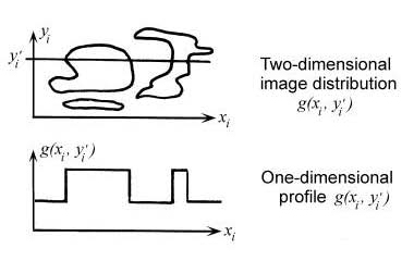
An object- or image-plane irradiance distribution is composed of "spatial frequencies" in the same way that a time-domain electrical signal is composed of various frequencies: by means of a Fourier analysis. As seen in Fig. 1.3, a given profile across an irradiance distribution (object or image) is composed of constituent spatial frequencies. By taking a one-dimensional profile across a two-dimensional irradiance distribution, we obtain an irradiance-vs-position waveform, which can be Fourier decomposed in exactly the same manner as if the waveform was in the more familiar form of volts vs time. A Fourier decomposition answers the question of what frequencies are contained in the waveform in terms of spatial frequencies with units of cycles (cy) per unit distance, analogous to temporal frequencies in cy/s for a time-domain waveform. Typically for optical systems, the spatial frequency is in cy/mm.
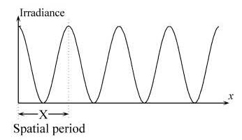
An example of one basis function for the one-dimensional waveform of Fig. 1.3 is shown in Fig. 1.4. The spatial period X (crest-to-crest repetition distance) of the waveform can be inverted to find the x-domain spatial frequency denoted by ξ ≡ 1/X.
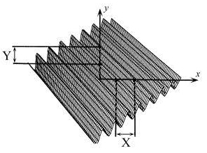
Fourier analysis of optical systems is more general than that of timedomain systems because objects and images are inherently two-dimensional, and thus the basis set of component sinusoids is also two-dimensional. Figure 1.5 illustrates a two-dimensional sinusoid of irradiance. The sinusoid has a spatial period along both the x and y directions, X and Y respectively. If we invert these spatial periods we find the two spatial frequency components that describe this waveform: ξ = 1/X and η = 1/Y. Two pieces of information are required for specification of the two-dimensional spatial frequency. An alternate representation is possible using polar coordinates, the minimum crest-to-crest distance, and the orientation of the minimum crest-to-crest distance with respect to the x and y axes.
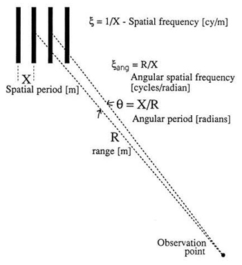
Angular spatial frequency is typically encountered in the specification of imaging systems designed to observe a target at a long distance. If the target is far enough away to be in focus for all distances of interest, then it is convenient to specify system performance in angular units, that is, without having to specify a particular range distance. Angular spatial frequency is most often specified in cy/mrad. It can initially be a troublesome concept because both cycles and milliradians are dimensionless quantities but, with reference to Fig. 1.6, we find that the angular spatial frequency ξang is simply the range R multiplied by the target spatial frequency ξ. For a periodic target of spatial period X, we define an angular period θ ≡ X/R, an angle over which the object waveform repeats itself. The angular period is in radians if X and R are in the same units. Inverting this angular period gives angular spatial frequency ξang= R/X. Given the resolution of optical systems, often X is in meters and R is in kilometers, for which the ratio R/X is then in cy/mrad.
G. D. Boreman, Modulation Transfer Function in Optical and Electro-Optical Systems, SPIE Press, Bellingham, WA (2001).
View SPIE terms of use.