Saddle points reveal essential properties of the merit-function landscape

In various areas of science and engineering, minimization of highly nonlinear functions with many variables is important. For instance, in optical-system design deviations from a given set of targets must be reduced by as much as possible within certain tolerances. Such a system is generally modeled as a point in multidimensional space in which the variables are constructional system parameters. Merit functions, i.e., functions that contain in a single number the defects of a specific configuration, typically have many local minima. Finding deep local minima, if possible the global minimum, is an essential part of the design process.

In the past decades, significant progress in the field of global optimization has led to development of powerful software packages for application to many design problems, including optics. Nevertheless, avoiding poor-quality local minima remains very challenging, particularly if the system is characterized by a large number of variables. The novel method of saddle-point construction (SPC) changes the dimensionality of the problem.¹ It can also be used successfully for very complex systems with many variables and constraints (e.g., in designing lithographic objectives²) because it enables generation of new system shapes with only a small number of local optimizations.

Figure 1. Derivation of two local minima with N+2 surfaces from a local minimum with N surfaces via a null-element saddle point (NESP).

In lens design, SPC is achieved by inserting lenses into the system. The approach works with any type of mirror or lens surface, but for simplicity we only discuss spherical surfaces. We start with an optimized system with N surfaces. Any optical merit function can be used, e.g., those based on transverse aberrations or wavefront distortions. In the existing system, i.e., a local minimum with N surfaces, we insert a meniscus lens of zero thickness and equal curvatures. This ‘null element’ disappears physically and affects neither the light path nor the system's merit function. However, if the new system is slightly modified, the new lens enables the merit function to decrease. There are two new variables, i.e., the two surface curvatures. For some specific curvature values the local minimum is transformed into a ‘saddle point’ in the variable space of increased dimensionality.¹

Figure 2. NESP characterized, at the position of insertion, by three surfaces with equal curvatures and with two zero distances. For clarity, the two zero distances are shown as small widths. The path of any ray (continuous line) is left unchanged by the null element.

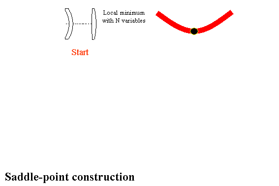
An intuitive illustration of SPC is shown in Figure 1. The starting system is minimum for all variables. For simplicity, only one variable is shown (in red) in the upper left of Figure 1. When the null element is added, new ‘downward’ (green) and ‘upward’ directions (not shown) appear in the new variable space (with dimension increased by 2). In the downward direction the new system shows a maximum and is therefore a ‘null-element’ saddle point (NESP). Although we typically have many more than two variables, the NESP resembles a 2D horse saddle. If we choose and optimize two points close to the NESP but on opposite sides of the saddle, the optimizations ‘roll down’ from the NESP and arrive at two distinct local minima. (The optimization variables are those of the initial local minimum and the two null-element curvatures.)

In general, if the insertion position and the glass of the null element are arbitrary, the curvature of the meniscus turning the system into an NESP can be computed numerically.³ An animation⁴ shows the system going through the phases of Figure 1. However, a simple and efficient version of the method occurs when the null element is inserted in contact with (i.e., at zero axial distance from) an existing surface—the reference surface—in the original local minimum. The type of glass of the null element should also be the same as that of the reference surface. In this special case, we can show that we obtain an NESP when the two curvatures of the null element (the second lens in Figure 2) are equal to that of the reference surface.¹ The conditions for insertion position and glass type are not as restrictive as they might seem, however. Once the minima on either side of the NESP have been obtained, the distances between the surfaces and the glass of the null-element lens can be changed as desired. SPC can be used in reverse order to remove lenses in a systematic way.

This new tool can increase design productivity. When a lens is inserted as usual, one new system shape results after optimization. However, when a lens is inserted with SPC, two distinct system shapes result, and for further design one can choose the optimal configuration. By inserting and (if required) removing lenses, new system shapes can be obtained very rapidly. The theory behind SPC is based on mathematical concepts which are still new in optical design, but the practical implementation is very easy, and the method can be fully integrated with all other traditional design tools.^5,6

In principle, SPC will also be applicable in other optimization problems satisfying certain mathematical conditions (i.e., the existence of two independent transformations of a null element that leave the merit function unchanged¹), e.g., in thin-film optimization. However, in applications other than lens design more research is needed to investigate the practical use of SPC. Work is presently being done to analyze SPC in a broader context, independent of lens design.